Cox Regression with Correlated Predictors

Yizeng Li

2025-10-28

Introduction

The glmsusie package implements the generalized sum of single effects (gSuSiE) model, which represents the overall effect as a sum of a small number of single-effect components. This approach extends variable selection to various regression models including Cox proportional hazards regression for survival analysis.

In this vignette, we demonstrate gSuSiE’s performance with survival outcomes and highly correlated predictors:

• Simulate a block-wise correlation structure with 100 predictors
• Apply gSuSiE to perform variable selection via glmsusie() with Cox regression
• Visualize coefficient estimates, posterior inclusion probabilities (PIPs), and credible sets (CSs)
• Evaluate predictive performance for survival analysis

Simulate data

We generate n=1000 observations and p=100 predictors with block-wise correlation. Every 10 consecutive variables are highly correlated (\rho=0.95) within each block, while blocks are independent. Only 4 variables have nonzero effects on the hazard, located in different correlation blocks.

set.seed(42)
n <- 1000     # sample size
p <- 100      # number of predictors
L <- 10       # number of single-effect components
block_size <- 10
n_blocks <- p / block_size
rho <- 0.95    # within-block correlation

# Create block-wise correlation matrix
Sigma <- matrix(0, p, p)
for (b in 1:n_blocks) {
  block_idx <- ((b-1)*block_size + 1):(b*block_size)
  # Within-block correlation matrix
  block_corr <- matrix(rho, block_size, block_size)
  diag(block_corr) <- 1
  Sigma[block_idx, block_idx] <- block_corr
}

# Generate correlated predictors
X <- MASS::mvrnorm(n, mu = rep(0, p), Sigma = Sigma)

# True sparse coefficients (one per block, spread across different blocks)
theta_true <- rep(0, p)
theta_true[c(3, 18, 47, 82)] <- c(1, -1, 1, -1)

# Generate survival data
library(survival)
linear_pred <- drop(X %*% theta_true)
hazard_ratio <- exp(linear_pred)

# Generate survival times from exponential distribution
lambda_baseline <- 0.1
survival_times <- rexp(n, rate = lambda_baseline * hazard_ratio)

# Generate censoring times (administrative censoring)
censor_times <- runif(n, min = 5, max = 15)

# Observed times and event indicators
observed_times <- pmin(survival_times, censor_times)
event_indicator <- as.numeric(survival_times <= censor_times)

# Create survival object
y <- Surv(observed_times, event_indicator)

cat("True nonzero coefficients at positions:", which(theta_true != 0), "\n")
## True nonzero coefficients at positions: 3 18 47 82
cat("True coefficient values:", theta_true[theta_true != 0], "\n")
## True coefficient values: 1 -1 1 -1
cat("Event rate:", mean(event_indicator), "\n")
## Event rate: 0.58
cat("Median follow-up time:", median(observed_times), "\n")
## Median follow-up time: 5.514619

Fit gSuSiE model

We allow up to L=10 single effects and use the Cox family for survival regression.

# Load glmsusie library
library(glmsusie)

# Model fitting
fit <- glmsusie(
  X      = X,
  y      = y,
  L      = L,
  family = cox()
)

summary(fit)
## 
## Call:
## glmsusie(X = X, y = y, L = L, family = cox())
## 
## Family: cox 
## 
## Coefficients: (sorted by PIP)
##          Estimate PIP
## X3   9.519446e-01   1
## X82 -9.357381e-01   1
## X47  9.215298e-01   1
## X18 -8.900653e-01   1
## X17 -1.283796e-02   0
## X15 -4.214844e-03   0
## X13 -3.411743e-03   0
## X50  1.738820e-08   0
## X12 -3.303270e-03   0
## X14 -3.423544e-03   0
## ... (90 more coefficients not shown)
## 
## 95% Confidence Sets:
##      Set Coverage
## cs1 {82}        1
## cs2  {3}        1
## cs3 {47}        1
## cs4 {18}        1
## 
## Model converged after 3 iterations.
## Computation time: 87.35 seconds.

Results

Coefficient estimates

The method successfully identifies the true signal locations despite high correlation within blocks:

plot(fit, which = "coefficients")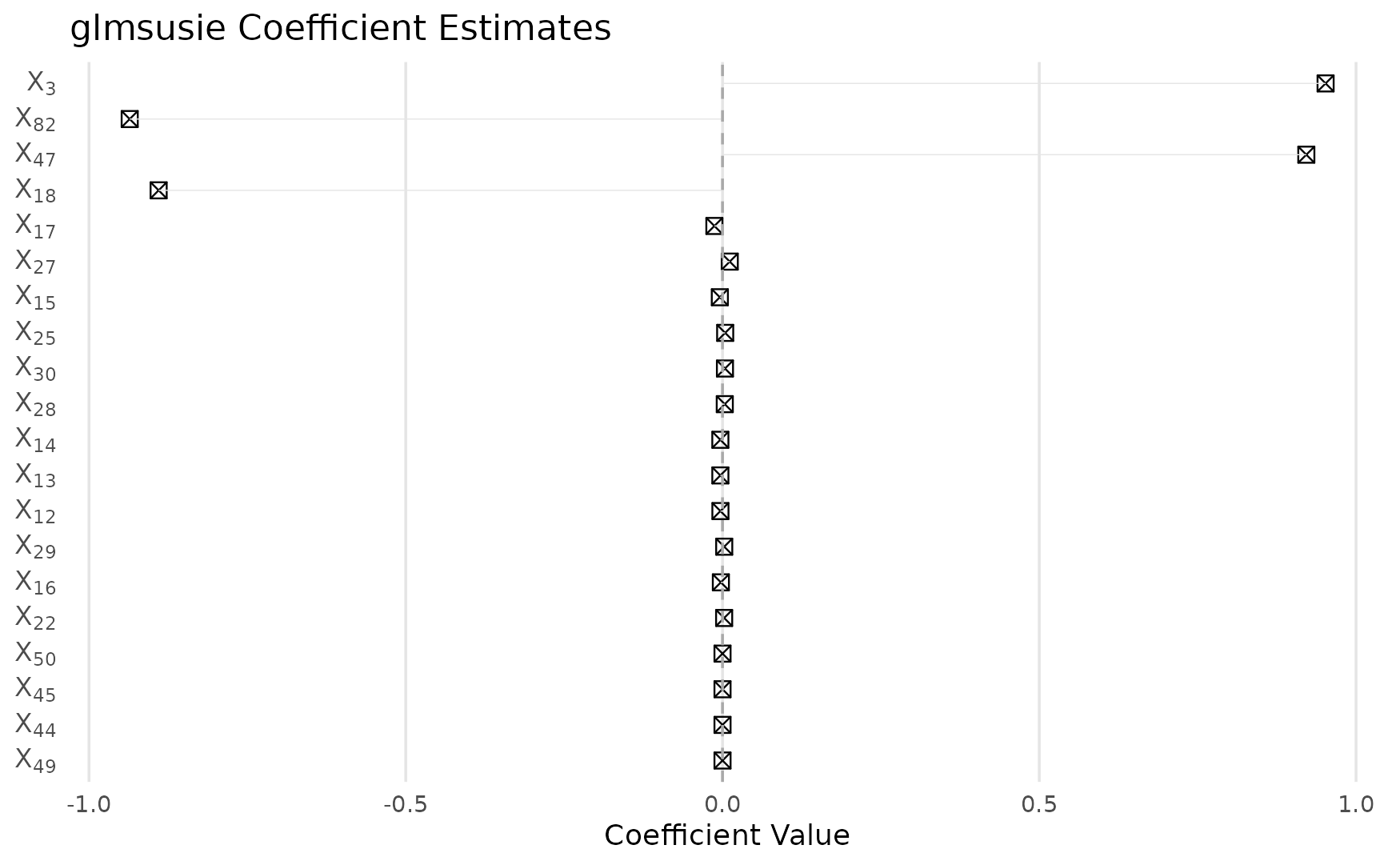

Posterior inclusion probabilities

Shows the probability that each variable is included in any single-effect component:

plot(fit, which = "probabilities")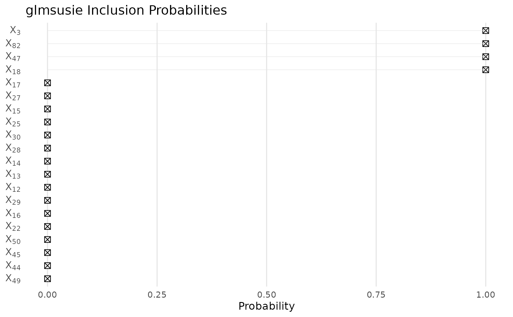

95% credible sets

Each credible set contains variables where at least one is likely active with 95% confidence. Note how the method handles correlated variables within blocks:

plot(fit, which = "sets")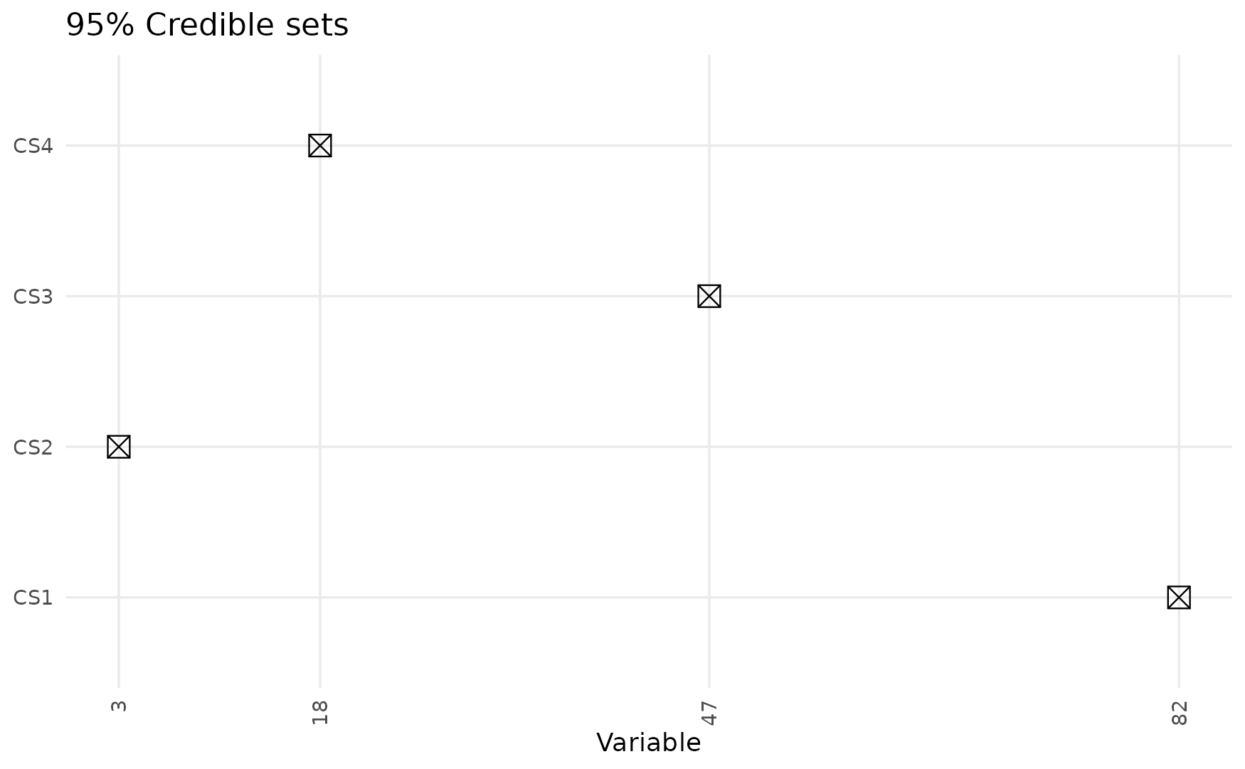

Credible sets summary

# Summary of credible sets
cs_sets <- fit$cs$sets
if (length(cs_sets) > 0) {
  cat("Number of credible sets:", length(cs_sets), "\n")
  for (i in seq_along(cs_sets)) {
    cat("CS", i, "contains variables:", cs_sets[[i]], "\n")
  }
  
  # Check coverage of true variables
  true_vars <- which(theta_true != 0)
  covered_vars <- intersect(unlist(cs_sets), true_vars)
  cat("\nTrue variables covered by credible sets:", covered_vars, "\n")
} else {
  cat("No credible sets identified\n")
}
## Number of credible sets: 4 
## CS 1 contains variables: 82 
## CS 2 contains variables: 3 
## CS 3 contains variables: 47 
## CS 4 contains variables: 18 
## 
## True variables covered by credible sets: 82 3 47 18

Coefficient comparison

Compare estimated coefficients with true values:

# Extract coefficients
coef_est <- coef(fit)
comparison <- data.frame(
  Variable = 1:p,
  True_Coef = theta_true,
  Estimated_Coef = coef_est,
  PIP = fit$pip
)

# Show results for true active variables
active_comparison <- comparison[theta_true != 0, ]
print(active_comparison)
##     Variable True_Coef Estimated_Coef       PIP
## X3         3         1      0.9519446 1.0000000
## X18       18        -1     -0.8900653 0.9999961
## X47       47         1      0.9215298 1.0000000
## X82       82        -1     -0.9357381 1.0000000

Conclusion

This example demonstrates that gSuSiE effectively handles Cox proportional hazards regression with highly correlated predictors. The method identifies relevant variables even when they are embedded within correlation blocks, providing both point estimates and uncertainty quantification through credible sets. The Cox family implementation successfully recovers the sparse signal structure in survival data while properly handling censoring and the semi-parametric nature of the Cox model.