Gaussian Linear Regression with Correlated Predictors

Yizeng Li

2025-10-28

Introduction

The glmsusie package implements the generalized sum of single effects (gSuSiE) model, which represents the overall effect as a sum of a small number of single-effect components. This approach extends the SuSiE method to generalized linear models.

In this vignette, we demonstrate gSuSiE’s performance with highly correlated predictors:

• Simulate a block-wise correlation structure with 100 predictors
• Apply gSuSiE to perform variable selection via glmsusie()
• Visualize coefficient estimates, posterior inclusion probabilities (PIPs), and credible sets (CSs)
• Compare performance against SuSiE

Simulate data

We generate n=5000 observations and p=100 predictors with block-wise correlation. Every 10 consecutive variables are highly correlated (\rho=0.98) within each block, while blocks are independent. Only 4 variables have nonzero effects, located in different correlation blocks.

set.seed(42)
n <- 5000     # sample size
p <- 100     # number of predictors
L <- 10      # number of single-effect components
block_size <- 10
n_blocks <- p / block_size
rho <- 0.98   # within-block correlation

# Create block-wise correlation matrix
Sigma <- matrix(0, p, p)
for (b in 1:n_blocks) {
  block_idx <- ((b-1)*block_size + 1):(b*block_size)
  # Within-block correlation matrix
  block_corr <- matrix(rho, block_size, block_size)
  diag(block_corr) <- 1
  Sigma[block_idx, block_idx] <- block_corr
}

# Generate correlated predictors
X <- MASS::mvrnorm(n, mu = rep(0, p), Sigma = Sigma)

# True sparse coefficients (one per block, spread across different blocks)
theta_true <- rep(0, p)
theta_true[c(3, 18, 47, 82)] <- c(1, -1, 1, -1)

# Generate response
y <- drop(X %*% theta_true + rnorm(n, sd = 3))

cat("True nonzero coefficients at positions:", which(theta_true != 0), "\n")
## True nonzero coefficients at positions: 3 18 47 82
cat("True coefficient values:", theta_true[theta_true != 0], "\n")
## True coefficient values: 1 -1 1 -1

Fit gSuSiE model

We allow up to L=10 single effects and use the default Gaussian family.

# Load glmsusie library
library(glmsusie)

# Model fitting
fit <- glmsusie(
  X      = X,
  y      = y,
  L      = L,
  family = gaussian()
)

summary(fit)
## 
## Call:
## glmsusie(X = X, y = y, L = L, family = gaussian())
## 
## Family: gaussian 
## 
## Coefficients: (sorted by PIP)
##        Estimate    PIP
## X82 -1.00455847 0.9999
## X47  0.99552173 0.9994
## X18 -0.90263767 0.9849
## X3   0.58003843 0.8059
## X4   0.08666866 0.2506
## X5   0.05426638 0.1618
## X1   0.04286195 0.1436
## X10  0.03441246 0.1262
## X6   0.03396987 0.1241
## X2   0.03030643 0.1160
## ... (90 more coefficients not shown)
## 
## 95% Confidence Sets:
##                              Set Coverage
## cs1                         {82}   0.9999
## cs2              {1, 3, 4, 5, 6}   0.9537
## cs3 {1, 2, 3, 4, 5, 6, 7, 9, 10}   0.9597
## cs4                         {47}   0.9994
## cs5                         {18}   0.9849
## 
## Model converged after 3 iterations.
## Computation time: 16 seconds.

Results

Coefficient estimates

The method successfully identifies the true signal locations despite high correlation within blocks:

plot(fit, which = "coefficients")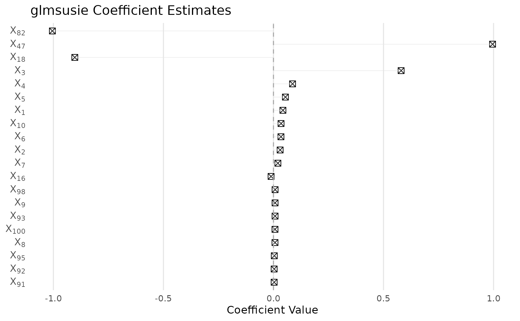

Posterior inclusion probabilities

Shows the probability that each variable is included in any single-effect component:

plot(fit, which = "probabilities")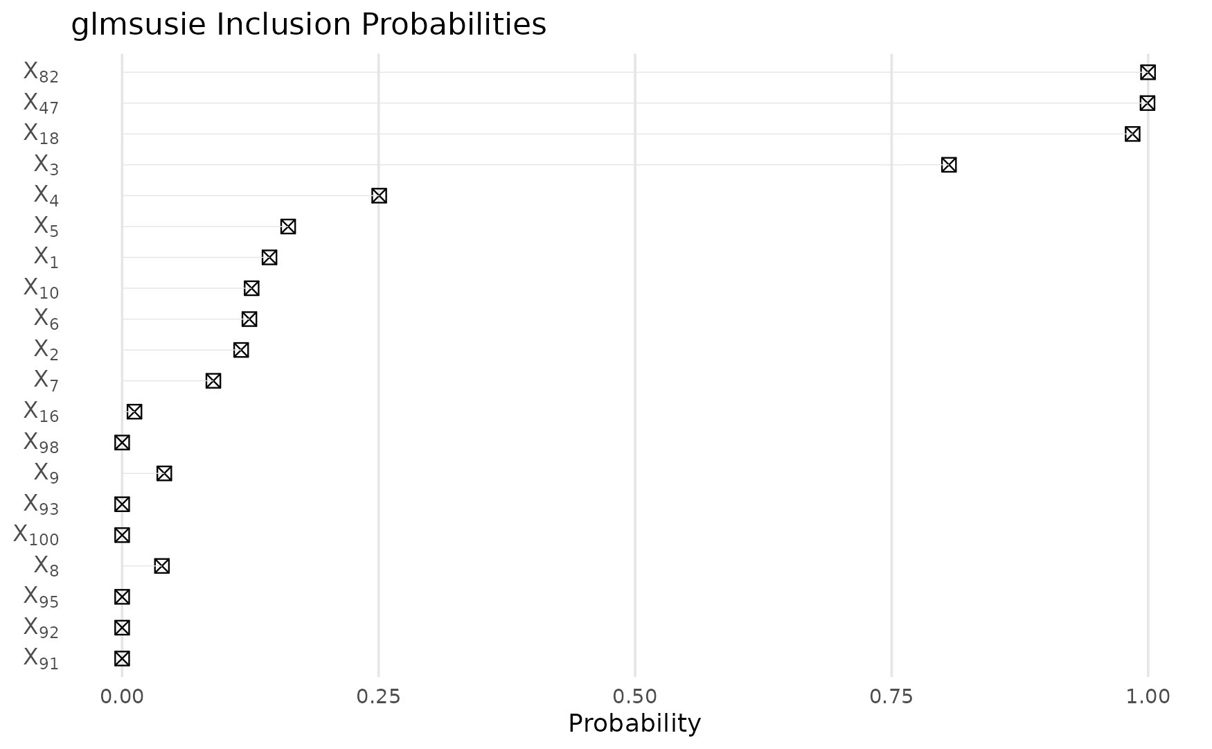

95% credible sets

Each credible set contains variables where at least one is likely active with 95% confidence. Note how the method handles correlated variables within blocks:

plot(fit, which = "sets")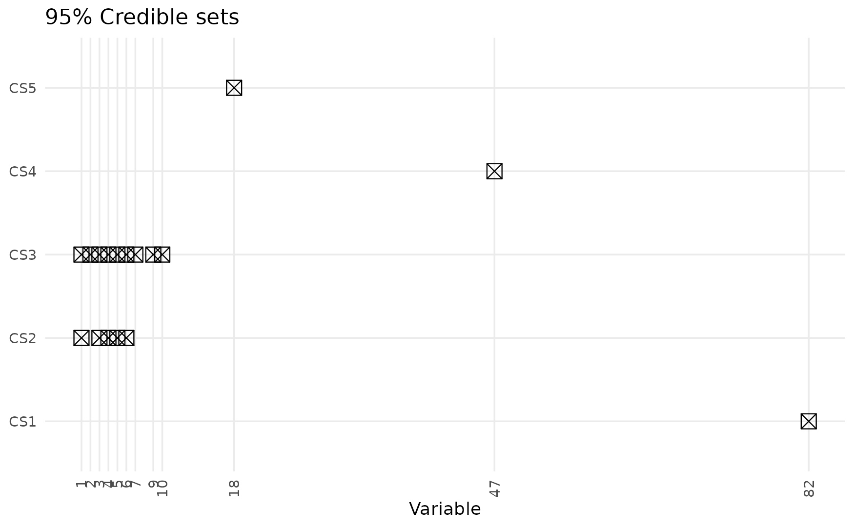

Performance evaluation

Compare predictive performance between methods:

# Prediction performance
rmse_glmsusie <- sqrt(mean(residuals(fit)^2))

# Compare with SuSiE
fit_susie <- susieR::susie(X, y, L = L)
fitted_susie <- fitted(fit_susie)
rmse_susie <- sqrt(mean((y - fitted_susie)^2))

performance <- data.frame(
  Method = c("SuSiE", "gSuSiE"),
  RMSE = c(rmse_susie, rmse_glmsusie)
)

print(performance)
##   Method     RMSE
## 1  SuSiE 3.008832
## 2 gSuSiE 3.009038

SuSiE credible sets comparison

Examine the credible sets identified by SuSiE:

# SuSiE credible sets
cat("SuSiE Credible Sets:\n")
## SuSiE Credible Sets:
susie_sets <- fit_susie$sets$cs
if (length(susie_sets) > 0) {
  for (i in seq_along(susie_sets)) {
    cs_vars <- susie_sets[[i]]
    cs_pips <- fit_susie$pip[cs_vars]
    
    # Format variables with their PIPs
    var_pip_strings <- paste0(cs_vars, " (PIP: ", round(cs_pips, 4), ")")
    
    cat("CS", names(susie_sets)[i], "contains variables:", 
        paste(var_pip_strings, collapse = ", "), "\n")
  }
} else {
  cat("No credible sets identified by SuSiE\n")
}
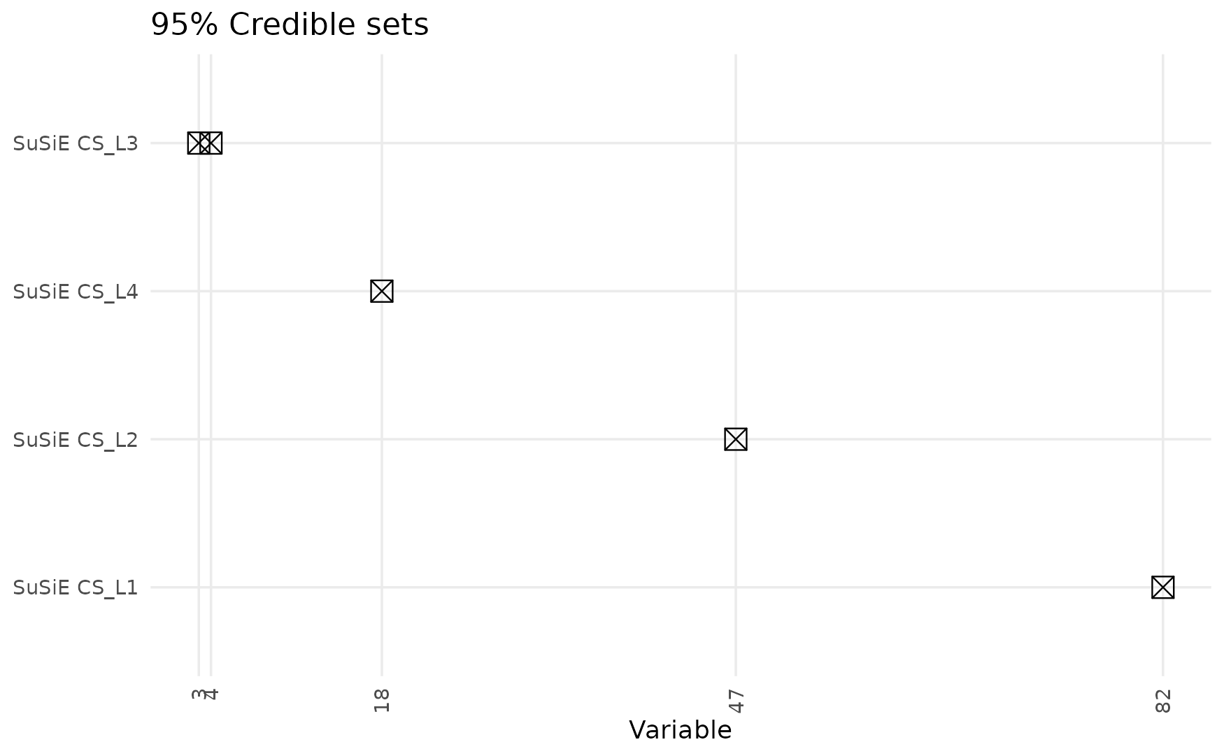
## CS L1 contains variables: 82 (PIP: 0.9999) 
## CS L2 contains variables: 47 (PIP: 0.9994) 
## CS L4 contains variables: 18 (PIP: 0.9848) 
## CS L3 contains variables: 3 (PIP: 0.7468), 4 (PIP: 0.2041), 5 (PIP: 0.028)

Visualize SuSiE credible sets

# Create matrix for SuSiE credible sets visualization
if (length(susie_sets) > 0) {
  # Create probability matrix for credible sets
  susie_cs_matrix <- matrix(0, nrow = length(susie_sets), ncol = p)
  
  for (i in seq_along(susie_sets)) {
    cs_vars <- susie_sets[[i]]
    # Use PIPs as probabilities for variables in the credible set
    susie_cs_matrix[i, cs_vars] <- fit_susie$pip[cs_vars]
  }
  
  # Plot SuSiE credible sets using our plotting function
  plot_cs_matrix(susie_cs_matrix, 
                 row_labels = paste0("SuSiE CS_", names(susie_sets)),
                 alpha = 0.05)
} else {
  cat("No SuSiE credible sets to visualize\n")
}

Conclusion

This example demonstrates that gSuSiE effectively handles very highly correlated predictors. The method identifies informative variables even when they are embedded within correlation blocks, providing both point estimates and uncertainty quantification through credible sets.