A Minimal Example

Introduction

The glmsusie package implements the generalized sum of single effects (gSuSiE) model, that represents the overall effect as a sum of a small number of single-effect components. In this vignette we:

Simulate a high-dimensional sparse linear regression dataset
Apply gSuSiE to perform variable selection via glmsusie()
Visualize coefficient estimates, posterior inclusion probabilities (PIPs), credible sets (CSs) and so on.
Evaluate predictive performance vs. SuSiE

Simulate data

We generate a sparse linear regression dataset with n=1000 observations and p=1000 predictors, where only 4 variables have nonzero effects.

set.seed(42)
n <- 1000    # sample size
p <- 1000    # number of predictors
L <- 10      # number of single-effect components

# true sparse coefficients
theta_true <- rep(0, p)
theta_true[c(100, 200, 300, 400)] <- 1

# covariate matrix and response
X <- matrix(rnorm(n * p), nrow = n, ncol = p)
y <- drop(X %*% theta_true + rnorm(n))

Fit the LASER model

We allow up to (L=10) single effects and use the default Gaussian family. Generally, this method is robust to larger L values and present minimal risk of overfitting.

# load glmsusie library
library(glmsusie)

# model fitting
fit <- glmsusie(
  X              = X,
  y              = y,
  L              = L,
  family         = gaussian()
)
summary(fit)
## 
## Call:
## glmsusie(X = X, y = y, L = L, family = gaussian())
## 
## Family: gaussian 
## 
## Coefficients: (sorted by PIP)
##       Estimate    PIP
## X300 1.0347174 1.0000
## X400 0.9491801 1.0000
## X100 0.9476146 1.0000
## X200 0.9745533 0.9997
## X1   0.0000000 0.0000
## X2   0.0000000 0.0000
## X3   0.0000000 0.0000
## X4   0.0000000 0.0000
## X5   0.0000000 0.0000
## X6   0.0000000 0.0000
## ... (990 more coefficients not shown)
## 
## 95% Confidence Sets:
##       Set Coverage
## cs1 {200}   0.9997
## cs2 {100}   1.0000
## cs3 {400}   1.0000
## cs4 {300}   1.0000
## 
## Model converged after 4 iterations.
## Computation time: 30.89 seconds.

Results

Coefficient estimates

We recover four peaks at the true locations

# plot coefficients
plot(fit, which="coefficients")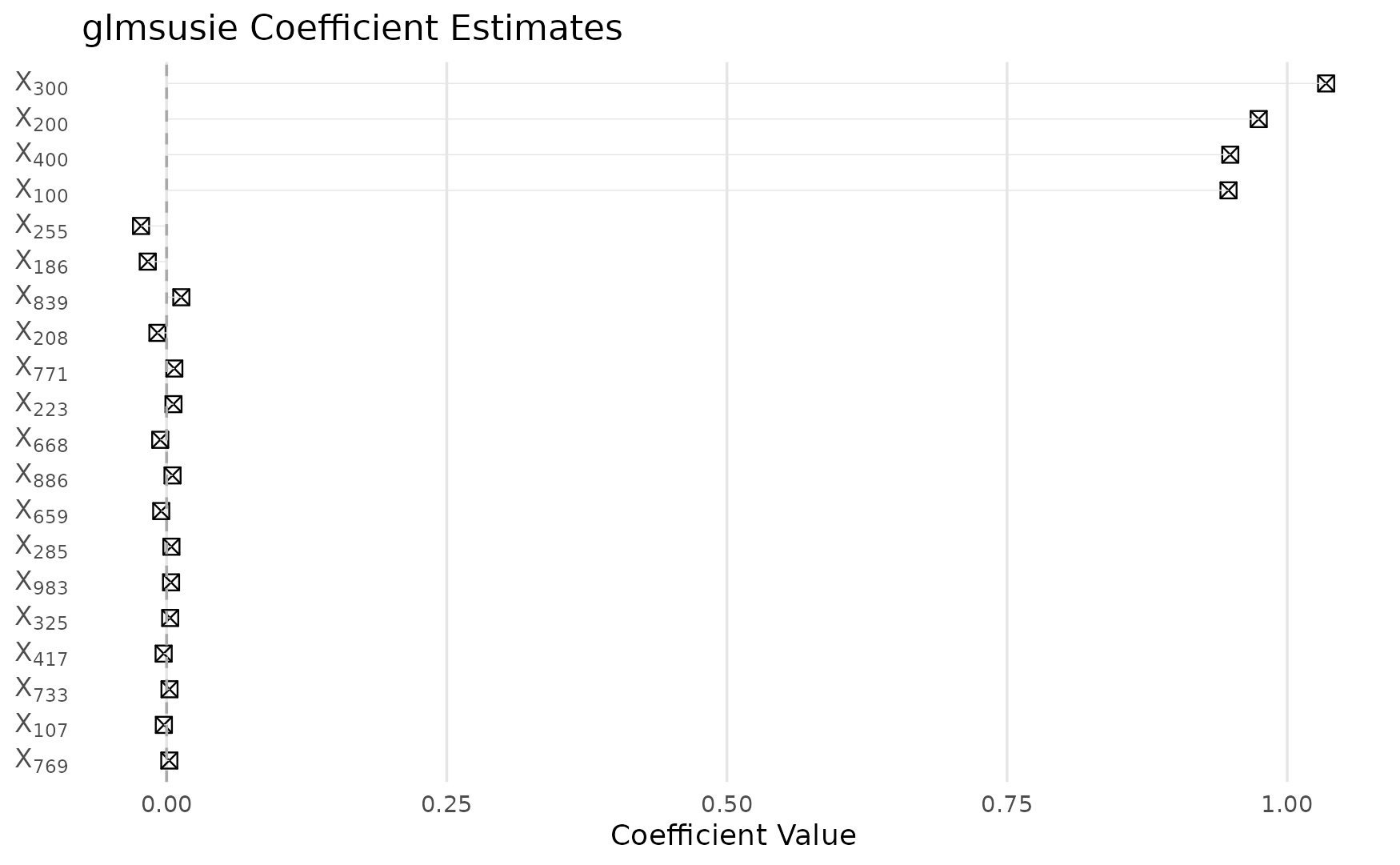

Estimated regression coefficients showing variable selection results.

Estimated inclusion probability

Shows the inclusion probability each variable is included in any single-effect component:

# plot coefficients
plot(fit, which="probabilities")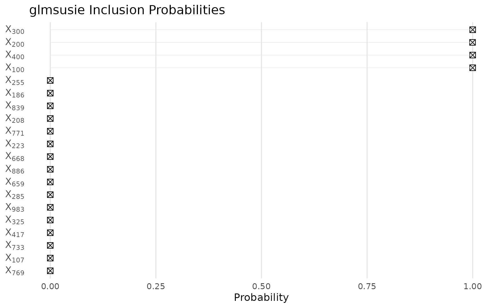

Posterior inclusion probabilities

Estimated 95% confidence sets

Each confidence set (CS) contains a small group of variables where at least one is likely to be active, with 95\% confidence.

# plot coefficients
plot(fit, which="sets")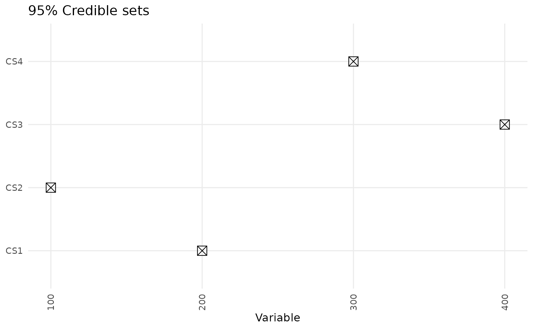

Credible sets

Performance evalution

rmse_glmsusie <- sqrt(mean(residuals(fit)^2))

# compare with SuSiE
fitted_susie  <- fitted(susieR::susie(X, y, L))
rmse_susie    <- sqrt(mean((y - fitted_susie)^2))

data.frame(
  Method = c("susie", "glmsusie"),
  RMSE   = c(rmse_susie, rmse_glmsusie)
)
##     Method      RMSE
## 1    susie 0.9728844
## 2 glmsusie 0.9609528

Yizeng Li

2025-10-28